In the last blog, we try to use linear regressions to model hospital admissions and vaccinations. The findings were the linear model tend to over-estimating how fast the admission rate is increasing on the higher range of vaccination rates, and residual variance is negatively correlated with vaccinations rates, suggesting heteroskedasticity. But it’s easy-peasy for Generalized linear models to fix those issues. GLM generalizes linear regression, 1. by allowing the linear model to be related to the response variable via a link function, 2. by allowing for the response variable to have an error distribution other than the normal distribution so that the magnitude of the variance of each measurement can change as a function of its predicted value.
Preliminaries
1 | import numpy as np |
The data I use includes hospital admissions and vaccinations from the CDC website, and the most up-to-date populations by state from the US Census Bureau.
1 | data_dir="../data" |
1 | hospitalizations=pd.read_csv(f"{data_dir}/covid_hospitalizations.csv",parse_dates=["date"]) |
| date | state | used_beds | admissions | vaccinated | population | |
|---|---|---|---|---|---|---|
| 0 | 2021-06-10 | MT | 66.0 | 16.0 | 0.397597 | 1080577 |
| 1 | 2021-06-21 | MT | 57.0 | 13.0 | 0.411614 | 1080577 |
| 2 | 2021-08-05 | MT | 149.0 | 23.0 | 0.440153 | 1080577 |
| 3 | 2021-07-15 | MT | 62.0 | 9.0 | 0.431722 | 1080577 |
| 4 | 2021-08-21 | MT | 224.0 | 59.0 | 0.449196 | 1080577 |
Poisson Regression
Like what we did with the linear regression, we can choose either to use the Poisson Regression model from statsmodels, or the GLM from the same lib. The two will give us the exact same estimations and statistics.
Model Definition
We have data from multiple dates, so it makes sense to incorporate Time as an extra variable.
\begin{eqnarray}
&\eta_i &=c + \beta_1 x_i + \beta_2 t_i + \beta_3 t_i^2 \newline
\mathbb{E}(y_i|x_i) =& \lambda_iP_i &= e^{\eta_i }P_i \newline
&p(y_i|x_i) & = \text{Poisson}(y;\lambda_i P_i)
\end{eqnarray}
where
- Each observation $i$ represents a single state at one particular date.
- $y_i$ is the number of hospital admissions on that state.
- $x_i$ is the percentage of the state population fully vaccinated that state.
- $t_i$ is the number of days elapsed since the beginning of the training period.
- $P_i$ is the population of the state.
- the parameters $c$ and $\beta_1,\beta_2,\beta_3$ will be fitted to the observed data to maximize agreement with the model
We including coefficients for $t$ and $t^2$ the dependence of the admission rate on time can have some curvature and does not need to be linear.
This can be fitter as a linear model where the inputs are $x_i$, $t_i$ and $t_i^2$
First we select the training period:
1 | start_train="2021-07-15" |
Then a 7-day testing period:
1 | test_period=7 # days |
1 | X_train,P_train=covid.define_variables(train_data,date0) |
Fit the model to the train data,
1 | mod=Poisson(Y_train,X_train,exposure=P_train.values) |
Optimization terminated successfully.
         Current function value: 32.115992
Iterations 6| Dep. Variable: | admissions | No. Observations: | 1632 |
|---|---|---|---|
| Model: | Poisson | Df Residuals: | 1628 |
| Method: | MLE | Df Model: | 3 |
| Date: | Sun, 26 Sep 2021 | Pseudo R-squ.: | 0.4493 |
| Time: | 19:44:49 | Log-Likelihood: | -52413. |
| converged: | True | LL-Null: | -95175. |
| Covariance Type: | nonrobust | LLR p-value: | 0.000 |
| coef | std err | z | P>|z| | [0.025 | 0.975] | |
|---|---|---|---|---|---|---|
| vaccinated | -6.7589 | 0.030 | -225.710 | 0.000 | -6.818 | -6.700 |
| T | 0.0750 | 0.001 | 75.492 | 0.000 | 0.073 | 0.077 |
| T2 | -0.0009 | 2.84e-05 | -31.349 | 0.000 | -0.001 | -0.001 |
| const | -8.4423 | 0.015 | -547.566 | 0.000 | -8.473 | -8.412 |
1 | mod=sm.GLM(Y_train,X_train,exposure=P_train,family=sm.families.Poisson(sm.families.links.log())) |
| Dep. Variable: | admissions | No. Observations: | 1632 |
|---|---|---|---|
| Model: | GLM | Df Residuals: | 1628 |
| Model Family: | Poisson | Df Model: | 3 |
| Link Function: | log | Scale: | 1.0000 |
| Method: | IRLS | Log-Likelihood: | -52413. |
| Date: | Sun, 26 Sep 2021 | Deviance: | 95443. |
| Time: | 19:44:50 | Pearson chi2: | 1.26e+05 |
| No. Iterations: | 6 | ||
| Covariance Type: | nonrobust |
| coef | std err | z | P>|z| | [0.025 | 0.975] | |
|---|---|---|---|---|---|---|
| vaccinated | -6.7589 | 0.030 | -225.710 | 0.000 | -6.818 | -6.700 |
| T | 0.0750 | 0.001 | 75.492 | 0.000 | 0.073 | 0.077 |
| T2 | -0.0009 | 2.84e-05 | -31.349 | 0.000 | -0.001 | -0.001 |
| const | -8.4423 | 0.015 | -547.566 | 0.000 | -8.473 | -8.412 |
Poisson regression is fit by maximum likelihood, there are several choices of Pseudo R-square
Here, what statsmodels implements for poisson regression is McFadden $R_{McF}^2$ that is defined as ratio of log likelihood for the fitted model and log likelihood of a model fitted to just a constant.
1 | # Pseudo R-squ McF |
0.44929536696336171 | res.llf, res.llnull |
(-52413.29834953645, -95174.97258108124)1 | 1-res.llf/res.llnull |
0.4492953669633617Certainly, we can implement other measures of the Pseudo R-square ourselves. Here I did $R_{L}^2$, which is deviance-based. It’s the most analogous index to the squared multiple correlations in linear regression. We will stick to it in our analysis from now on.
1 | def poisson_deviance(y,y_pred): |
1 | mu_train=Y_train.sum()/P_train.sum() |
0.4725915412837366If you don’t want bother yourself with the mathematical formulas, here’s a simpler way (my favorite as the laziest person ever). Just fit the model with a constant, and take the log-likelihood/deviance as your null case.
1 | mod=sm.GLM(Y_train,X_train['const'],exposure=P_train,family=sm.families.Poisson(sm.families.links.log())) |
180966.735525515221 | # null deviance from our math formula |
180966.7355255152After all, the R-squared we have for now is 0.473.
Next let’s check on how the model predicts.
Extrapolation of Time trends
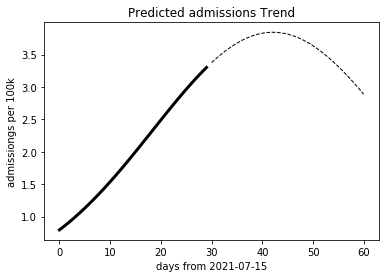
Remember what we saw last time with the linear model? Its projection was a straight line. But the poisson model is telling us a different story, that the admissions will flatten out assuming the current vaccination rate. Well, it is onto something, isn’t it?
1 | covid.plot_time_extrapolation(train_data,glm_res,event,date0) |
In-sample model Fit
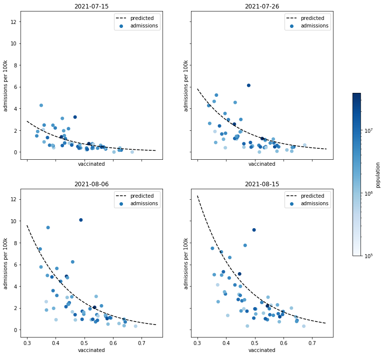
To better evaluate the model fit, we visualize the real observations and model predictions. Here’s some snapshots of the fit for a few selected dates on the training period.
As we can see, curves from the poisson regression model fits the data much better than the linear model, indicating the correlation between admissions and vaccinations are not linear.
1 | covid.plot_time_facets(train_data,glm_res,event,date0) |
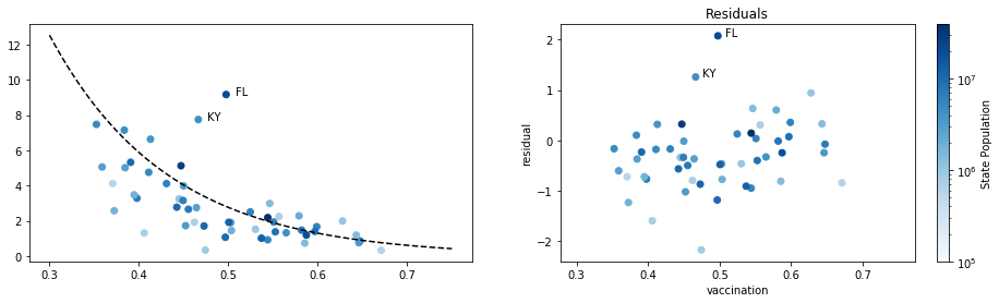
But is this enough? Certainly not, let’s verify the deviance residuals by visualizing them,
1 | def plot_deviance_residuals(data,event,res): |
The date I choose is Aug.15,
1 | offset=9 |
1 | plot_deviance_residuals(interested_data,event,glm_res) |
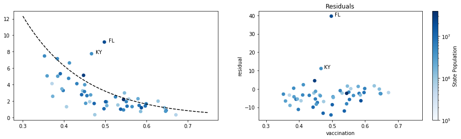
The deviance residuals are defined as the signed square roots of the unit deviances, representing the contributions of individual samples to the deviance. The deviance indicates the extent to which the likelihood of the saturated model exceeds the likelihood of the proposed model. If the proposed model has a good fit, the deviance will be small. If the proposed model has a bad fit, the deviance will be high.
Thus, the deviance residuals are analogous to the conventional residuals: when they are squared, we obtain the sum of squares that we use for assessing the fit of the model. However, while the sum of squares is the residual sum of squares for linear models, for GLMs, this is the deviance.
1 | deviance=poisson_deviance(Y_train,Y_pred) |
(95443.38706242564, 95443.38706242583)In a properly specified model, the deviance is approximately chi-square distributed with n-k-1 degrees of freedom, and the deviance residuals would be independent, standard normal random variables, i.e., ~ norm(0,1). So we would expect the residuals to be mostly in range of -1 to 1, and rarely fall outside the ± 3 limits.
However, the model residuals are 10 times larger than expected and we say there is overdispersion. If overdispersion is present in a dataset, the estimated standard errors and test statistics, the overall goodness-of-fit will be distorted and adjustments must be made.
A more appropriate model will be a Negative Binomial regression.
Model Prediction
We will now use the model without recalibrating to make predictions about admission rates on new data.
This is out of sample evaluation. It is the only way to make sure the model really works.
Out of Sample $R^2$
1 | test_admission_mean=Y_test.sum()/P_test.sum() |
0.371917369051069Out of sample $R^2$ is worse than for the in sample (approx. 0.473). I think we’ll all agree, predicting the future is hard.
Negative Binomial Regression
Model Definition
We have data from multiple dates, so it makes sense to incorporate Time as a extra variable.
\begin{eqnarray}
&\eta_i &=c + \beta_1 x_i + \beta_2 t_i + \beta_3 t_i^2 \newline
\mathbb{E}(y_i|x_i) =& \lambda_i P_i &= e^{\eta_i } P_i \newline
&p(y_i|x_i) & = \text{NB}(y_i; \lambda_i P_i, \alpha)
\end{eqnarray}
where
- Each observation $i$ represents a single state at one particular date.
- $y_i$ is the number of hospital admissions on that state.
- $x_i$ is the percentage of the state population fully vaccinated that state.
- $t_i$ is the number of days elapsed since the beginning of the training period.
- $P_i$ is the population of the state.
- the parameters $c$ and $\beta_1,\beta_2,\beta_3$ will be fitted to the observed data to maximize agreement with the model
We including coefficients for $t$ and $t^2$ the dependence of the admission rate on time can have some curvature and does not need to be linear.
This can be fitter as a linear model where the inputs are $x_i$, $t_i$ and $t_i^2$
Variance Comparison to Poisson Model
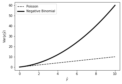
Introducing a free additional parameter $\alpha$ give more accurate models than simple parametric models like the Poisson distribution by allowing the mean and variance to be different, unlike the Poisson. The negative binomial distribution has a variance $\hat{y}+\hat{y}^2\alpha$ . This can make the distribution a useful overdispersed alternative to the Poisson distribution.
As we can see, with an extra parameter $\alpha$ to control the variance, the expected variance of observations is larger with the Negative Binomial Model than with the Poisson model.
1 | alpha = 0.5 |
Choosing $\alpha$
Negative Binomial is a GLM model with an extra parameter $\alpha$ that we must choose by maximizing the log likelihood.
The train/test data we fit to the Negative Binomial Regression is the same as what we create at start.
1 | lls=[] |
alpha 0.3004008016032064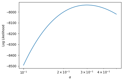
The best alpha is 0.3004 given a run of 500 times. Or easier, we can go for the Negative Regression model from statsmodels, which can do the dirty work, optimizing alpha for us.
1 | #mod=sm.GLM(Y_train,X_train,exposure=P_train,family=nb) |
/opt/anaconda3/lib/python3.7/site-packages/statsmodels/discrete/discrete_model.py:2642: RuntimeWarning: divide by zero encountered in log
  llf = coeff + size*np.log(prob) + endog*np.log(1-prob)
/opt/anaconda3/lib/python3.7/site-packages/statsmodels/discrete/discrete_model.py:2642: RuntimeWarning: invalid value encountered in multiply
  llf = coeff + size*np.log(prob) + endog*np.log(1-prob)
/opt/anaconda3/lib/python3.7/site-packages/statsmodels/base/model.py:568: ConvergenceWarning: Maximum Likelihood optimization failed to converge. Check mle_retvals
ConvergenceWarning)| Dep. Variable: | admissions | No. Observations: | 1632 |
|---|---|---|---|
| Model: | NegativeBinomial | Df Residuals: | 1628 |
| Method: | MLE | Df Model: | 3 |
| Date: | Sun, 26 Sep 2021 | Pseudo R-squ.: | 0.08843 |
| Time: | 20:24:21 | Log-Likelihood: | -7946.2 |
| converged: | False | LL-Null: | -8717.1 |
| Covariance Type: | nonrobust | LLR p-value: | 0.000 |
| coef | std err | z | P>|z| | [0.025 | 0.975] | |
|---|---|---|---|---|---|---|
| vaccinated | -6.7968 | 0.179 | -38.019 | 0.000 | -7.147 | -6.446 |
| T | 0.0525 | 0.006 | 8.645 | 0.000 | 0.041 | 0.064 |
| T2 | -0.0002 | 0.000 | -1.262 | 0.207 | -0.001 | 0.000 |
| const | -8.4877 | 0.092 | -92.109 | 0.000 | -8.668 | -8.307 |
| alpha | 0.3025 | 0.011 | 26.621 | 0.000 | 0.280 | 0.325 |
The alpha values are close,
1 | p=res.params |
0.3024936677385029Compared to Poisson:
- The regression coefficients are very similar.
- The confidence intervals are much wider.
- The t statistics are smaller because we assume a larger variance of residuals.
In summary, switching from Poisson to Negative Binominal yields stable coefficient estimates, but a higher chance for the null hepothesis to be rejected and more reliable confidence intervals.
The statsmodel.family.NegativeBinomial object knows how to compute deviance, and we use it to calculate the R squared,
1 | mu_train=Y_train.sum()/P_train.sum() |
0.5937123540474427In-sample model Fit
1 | covid.plot_time_facets(train_data,res,event,date0) |
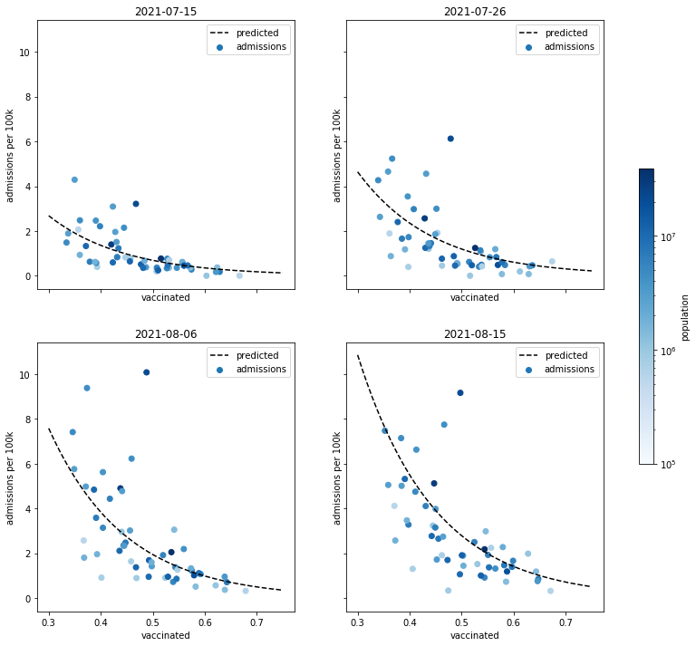
Then most excitingly, let’s check out the deviance residuals again. The residuals are now well behaved, randomly fall into the range of -1 to 1. Though FL, KY and a few other states seem to be outliers. But no worries, we will address them in our next blog, using a more advanced method - mixed models.
1 | plot_deviance_residuals(interested_data,event,glm_res) |
Model Prediction
Finally, always take a look at the out-of-sample fit.
Though the R squared is not as good as the in-sample, but there’s still an improvement comparing to Poisson regression and the linear regressions.
1 | test_admission_mean=Y_test.sum()/P_test.sum() |
0.4595499732848517