Lately I’ve been working on a project predicting credit losses for mortgages with a bunch of loan-level attributes. To be honest, the data wasn’t rich. In pursuit of good predictive power, I had to try from the simple multi-period regression, to generalized linear model with distributions beyond the Gaussian family, then mixed effect models, and even used some curve fitting techniques like splines at last to fix the oversimple (or wrong) assumptions I made at the beginning. Overall, I think the journey was inspiring as it basically shows that one can almost crack any problem with regression analysis, more importantly, in an elegant way.
When it comes to predictive modeling, people always turn to linear regressions, which isn’t wrong, just so you know that linear regression models and OLS make a number of assumptions about the predictor variables, the response variable, and their relationship. Violating these assumptions can result in biased predictions or imprecise coefficients, in short cause your model to be less predictive. Well, the good news is that there are numerous extensions have been developed that allow each of these assumptions to be relaxed, and in some cases eliminated entirely, but only if you know what they are and when to use them. More commonly, I see people get stuck and choose to live with a just-fine-fit model without knowing that they can easily fix it by employing a more generalized regression models. Now let’s see how powerful regressions can get through a trendy modeling case - project covid admissions based on the vaccinate progress.
Preliminaries
1 | import numpy as np |
The data I use includes hospital admissions and vaccinations from the CDC website, and the most up-to-date populations by state from the US Census Bureau.
1 | data_dir="../data" |
1 | hospitalizations=pd.read_csv(f"{data_dir}/covid_hospitalizations.csv",parse_dates=["date"]) |
| date | state | used_beds | admissions | vaccinated | population | |
|---|---|---|---|---|---|---|
| 0 | 2021-06-10 | MT | 66.0 | 16.0 | 0.397597 | 1080577 |
| 1 | 2021-06-21 | MT | 57.0 | 13.0 | 0.411614 | 1080577 |
| 2 | 2021-08-05 | MT | 149.0 | 23.0 | 0.440153 | 1080577 |
| 3 | 2021-07-15 | MT | 62.0 | 9.0 | 0.431722 | 1080577 |
| 4 | 2021-08-21 | MT | 224.0 | 59.0 | 0.449196 | 1080577 |
Now we are good to go. As always, let’s first check on our old friend, simple linear regression with one single explanatory variable, as a warm-up.
Here specifically, I am using weighted least squares rather than ordinary least squares to incorporate the knowledge of state populations. WLS is a generalization of OLS and a specialization of generalized least squares, which can relax the assumptions of constant variance, allowing the variances of the observations to be unequal i.e., heteroscedasticity (btw one of my favorite words in statistics, the pronunciation’s fun).
Single Period Regression
Model Definition
The weighted linear regression model is defined as:
\begin{eqnarray}
\hat{y}_i &= c + \beta x_i \newline
y_i &=\hat{y}_i+ \epsilon_i \newline
\end{eqnarray}
and we minimize the weighted least squares error :
\begin{equation}
E_w = \sum_i P_i(y - \hat{y}_i)^2
\end{equation}
where
- Each observation $i$ represents a single state.
- $\hat{y}_i$ is the predicted probability of hospital admissions per persons on that state.
- $y_i$ is the actual number of events per person observed.
- $x_i$ is the percentage of the state population fully vaccinated.
- $P_i$ is the population of the state.
- $\epsilon_i$ is a Gaussian uncorrelated noise with constant variance $\sigma$
- the parameters $c$ and $\beta$ will be fitted to the observed data to maximize agreement with the model
We first fit the regression model to single day of state hospitalization data.
1 | offset=9 # if we do not want to look at the last day, subtract here. |
Let’s take Aug.15,
1 | last_date=data["date"].max()-pd.offsets.Day(offset) |
1 | X=sm.add_constant(last_data["vaccinated"]) |
Use statmodels for Weighted Linear Regression
Let’s first use the Weighted Linear Regression model from statmodels.
The exact same estimation can be done by a different way, which I will show later.
1 | mod=sm.WLS(Y,X,P) |
const         0.000127
vaccinated   -0.000190
dtype: float64
So here’s our estimation of the coefficients and some statistics that are helpful for diagnosis. It’s easy to read that the R-squared is 0.327. But we can also calculate it ourselves.
The R-square is defined as ratio of square loss to target variance,
1 | def square_error(y,y_hat,P): |
1 | Y_pred=res.predict(X) |
0.3266337795171833Use statmodels GLM for Weighted Linear Regression
Exactly the same model can be written in the more general language of Generalized Linear models as
Model Definition
The linear regression model is defined as:
\begin{eqnarray}
&\eta_i &=c + \beta*x_i \newline
\mathbb{E}(y_i|x_i) =& \hat{y}_i &= \eta_i \newline
&p(y_i|x_i) & = N(\hat{y}_i,\sigma)
\end{eqnarray}
The fact that $\eta_i=\hat{y}_i$ means we are using the identity link between the Gaussian family and the linear model $\eta$. One should be aware here that linear model is just a specical case of GLM.
1 | glm_model=sm.GLM(Y,X,family=sm.families.Gaussian(sm.families.links.identity()),var_weights=P) |
const         0.000127
vaccinated   -0.000190
dtype: float64
Results are the same. But with the GLM language we will be able to perform regression many more kinds of variables.
The generalization of square error for a GLM model is called the deviance. This is the square error the Gaussian Family used in linear regression. Let’s calculate the in-sample R-squared in the GLM way and compare it with the previous.
1 | glm_res.deviance, square_error(Y,Y_pred,P) |
(0.12246143037040369, 0.12246143037040369)The resuls also include the deviance for the null model fitted to just a constant
1 | glm_res.null_deviance,square_error(Y,Y_bar,P) |
(0.1818645287591, 0.1818645287591)The ratio defines an $R^2$ value. Not surprisingly, the results are exactly the same. Overall, I admit a 32.7% R-squared model can barely be said to be a good model. But no worries, all can be fixed.
1 | 1-glm_res.deviance/glm_res.null_deviance |
0.3266337795171833Now, as we have a better understanding of the data and the modeling methodologies, let’s move on to model the time series.
The data we have here is time series data, indeed panel data, as time series and cross-sectional data are both special cases of panel data that are in one dimension only. But we will deal with the multi-subjects matter in the next blog(probably should have a spoiler tag oops). Anyways, let’s first start with the multi-period regression, here I have trend variables added to the model to represent time.
Multiple Period Regression
Model Definition
\begin{eqnarray}
&\eta_i &=c + \beta_1 x_i + \beta_2 t_i + \beta_3 t_i^2 \newline
\mathbb{E}(y_i|x_i) =& \hat{y}_i &= \eta_i \newline
&p(y_i|x_i) & = N(\hat{y_i},\sigma^2)
\end{eqnarray}
where
- Each observation $i$ represents a single state at one particular date.
- $y_i$ is the number of events on that state.
- $\hat{y}_i$ is the predicted number of events on that state.
- $x_i$ is the percentage of the state population fully vaccinated on that state.
- $t_i$ is the number of days elapsed since the beginning of the training period.
- $\sigma^2$ is the level of noise of the observations (the variance of the residuals).
- the parameters $c$ and $\beta_1,\beta_2,\beta_3$ will be fitted to the observed data to maximize agreement with the model
This can be fitter as a linear model where the inputs are $x_i$, $t_i$ and $t_i^2$
First we select the training period:
1 | start_train="2021-07-15" |
Then a 7-day testing period:
1 | test_period=7 # days |
I write a function to generate the desired matrix,
1 | def define_variables(data,date0): |
1 | X_train,P_train=covid.define_variables(train_data,date0) |
Weighted Multi-period Linear Regression
1 | mod=sm.WLS(Y_train,X_train,P_train) |
| Dep. Variable: | y | R-squared: | 0.373 |
|---|---|---|---|
| Model: | WLS | Adj. R-squared: | 0.371 |
| Method: | Least Squares | F-statistic: | 322.3 |
| Date: | Tue, 21 Sep 2021 | Prob (F-statistic): | 3.12e-164 |
| Time: | 15:16:26 | Log-Likelihood: | 15151. |
| No. Observations: | 1632 | AIC: | -3.029e+04 |
| Df Residuals: | 1628 | BIC: | -3.027e+04 |
| Df Model: | 3 | ||
| Covariance Type: | nonrobust |
| coef | std err | t | P>|t| | [0.025 | 0.975] | |
|---|---|---|---|---|---|---|
| vaccinated | -0.0002 | 6.13e-06 | -24.647 | 0.000 | -0.000 | -0.000 |
| T | 1.038e-06 | 1.82e-07 | 5.686 | 0.000 | 6.8e-07 | 1.4e-06 |
| T2 | -1.18e-09 | 5.69e-09 | -0.207 | 0.836 | -1.23e-08 | 9.98e-09 |
| const | 8.1e-05 | 3.17e-06 | 25.544 | 0.000 | 7.48e-05 | 8.72e-05 |
| Omnibus: | 1418.486 | Durbin-Watson: | 0.372 |
|---|---|---|---|
| Prob(Omnibus): | 0.000 | Jarque-Bera (JB): | 43359.192 |
| Skew: | 4.022 | Prob(JB): | 0.00 |
| Kurtosis: | 26.936 | Cond. No. | 6.93e+03 |
Notes:
[1] Standard Errors assume that the covariance matrix of the errors is correctly specified.
[2] The condition number is large, 6.93e+03. This might indicate that there are
strong multicollinearity or other numerical problems.
Calculate the R-squared again, still, not good enough.So let's take a deep dive and see where can be improved.
1 | Y_bar=np.sum(Y_train*P_train)/np.sum(P_train) # weighted average |
0.3726019173009557Extrapolation of Time trends
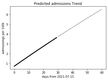
The linear model projects the admission to be increasing steadily if assuming current vaccination rate.
1 | covid.plot_time_extrapolation(train_data,res,event,date0) |
In-sample model Fit
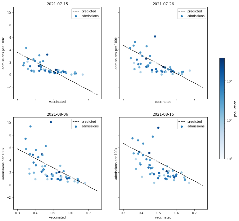
To better evaluate the model fit, we visualize the real observations and model prodictions. Here’s some snapshots of the fit for a few selected dates on the training period.
Observations are arranged by state and date.
Don’t have to say much, you can tell the weighted linear model doesn’t fit well as the corelation between vaccinations and admissions looks more like a curve than a straight line.
1 | covid.plot_time_facets(train_data,res,event,date0) |
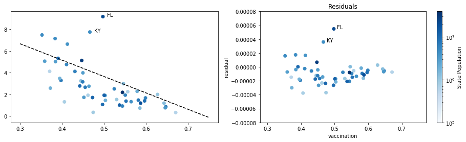
We can further plot out the residuals. I choose one date from the dates above, Aug.15 and apply the following function to generate its residual plot.
1 | def plot_residuals(data,event,res): |
We can see that
- Predicted events can be negative for large vaccination rates, saying we are over estimating how fast the admission rate is increasing.
- residual variance is negatively correlated with vaccinations rate i.e., smaller vaccination rates have larger magnitude residuals. A Poisson model can fix those issues, which will be the topic of our next blog.
- Some states like FL and KY look like outliers, indicating that they may have different intercepts than the others, which is not surprising as states are different subjects and each may have unique fundamentals. A mixed model would be a good solution for this.
1 | plot_residuals(last_data,event,res) |
Model Prediction
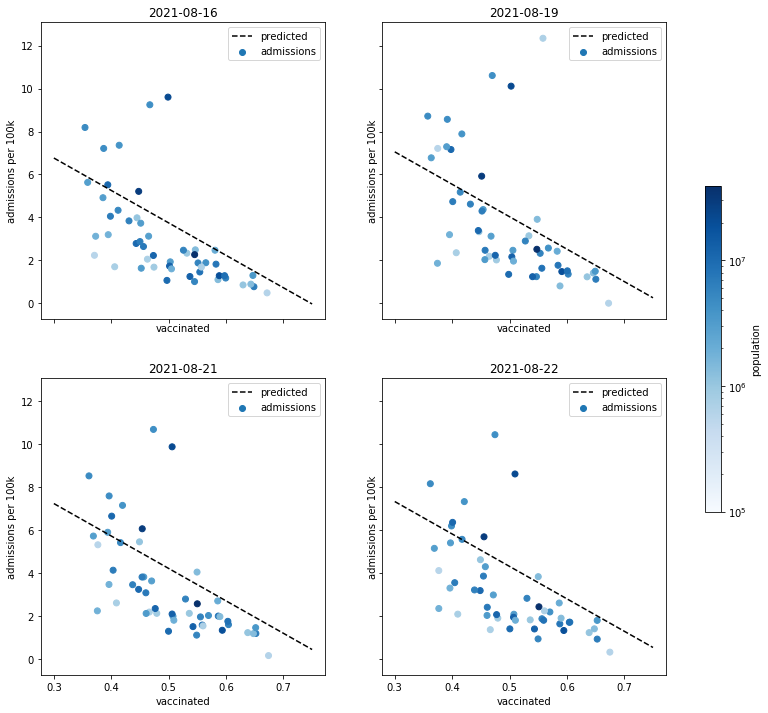
We will now use the model without recalibrating to make predictions about admission rates on new data.
This is out of sample evaluation. It is the only way to make sure the model really works.
Out of Sample Model Fit
Besides greater residuals, the out of sample evaluation is basically telling us a same story.
1 | covid.plot_time_facets(test_data,res,event,date0) |
Day of the Week Effects
Before we move on to GLM, there’s another trick to play with. The data reporting obviously has day of the week effects,
1 | aggregate=data.groupby(["date"])[event].sum() |
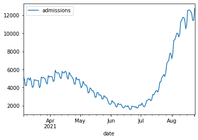
We use a new function to generate the train data, more dummy variables are added to represent days of a week,
1 | def define_variables2(data,date0): |
1 | X_train,P_train=define_variables2(train_data,date0) |
| vaccinated | T | T2 | const | Monday | Saturday | Sunday | Thursday | Tuesday | Wednesday | |
|---|---|---|---|---|---|---|---|---|---|---|
| 2 | 0.440153 | 21 | 441 | 1.0 | 0 | 0 | 0 | 1 | 0 | 0 |
| 3 | 0.431722 | 0 | 0 | 1.0 | 0 | 0 | 0 | 1 | 0 | 0 |
| 6 | 0.435852 | 10 | 100 | 1.0 | 0 | 0 | 1 | 0 | 0 | 0 |
| 8 | 0.441906 | 24 | 576 | 1.0 | 0 | 0 | 1 | 0 | 0 | 0 |
| 10 | 0.437877 | 15 | 225 | 1.0 | 0 | 0 | 0 | 0 | 0 | 0 |
1 | mod=sm.WLS(Y_train,X_train,P_train) |
vaccinated   -1.510900e-04
T             1.028112e-06
T2           -6.639196e-10
const         8.186223e-05
Monday       -2.235516e-06
Saturday     -8.318830e-07
Sunday       -3.189080e-06
Thursday     -2.233662e-08
Tuesday       3.232847e-07
Wednesday    -2.672040e-07
dtype: float64
1 | res.rsquared |
0.37572844250241666$R^2$ is 0.376, higher than the 0.373 we previously have. Day of the week provides a small improvement on $R^2$ compared to original model.